SWMM Calibration Workflow for Small Subdivision Drainage Studies

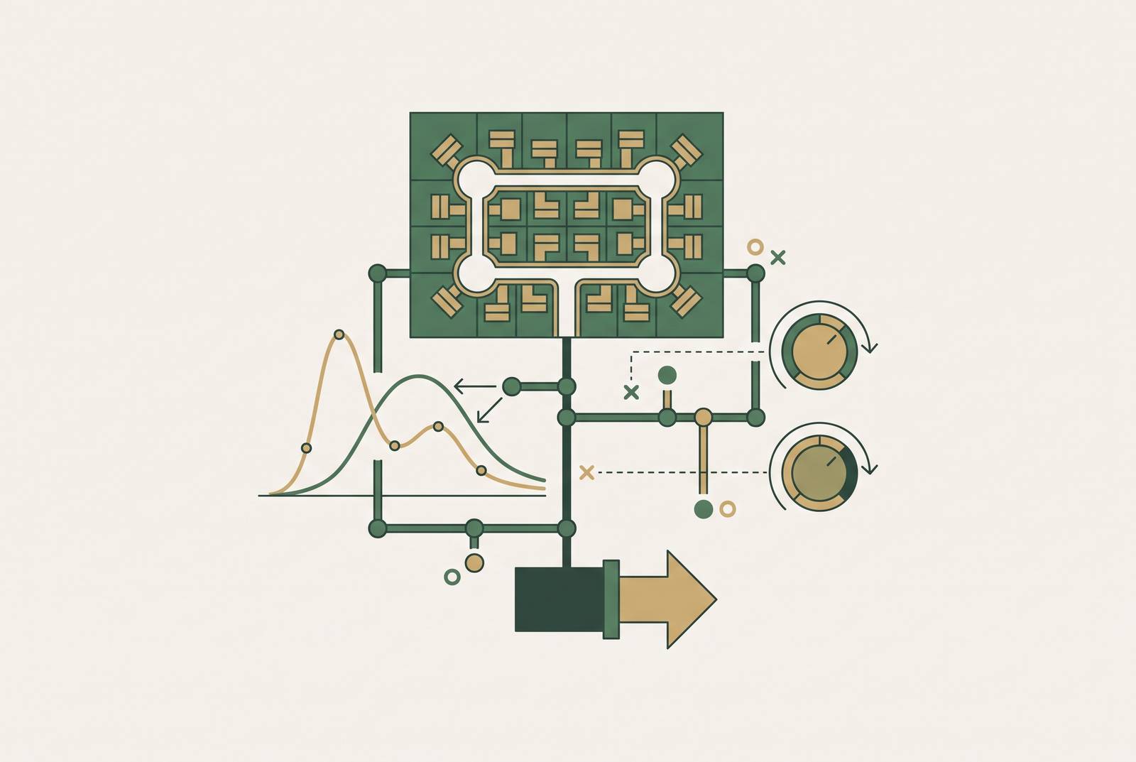
SWMM calibration fails at subdivision scale when you treat it as a scaled-down version of large-watershed practice. The parameters that govern a 27.5-hectare low-density development behave differently than those in a dense urban catchment, and guessing which ones matter produces models that look calibrated but fall apart under review. A defensible subdivision model follows a specific sequence: diagnose the impervious fraction, rank parameters by sensitivity, narrow their ranges, iterate against observed storms, validate against withheld events, and document every decision.

Why SWMM calibration for small subdivisions is its own problem

The central difficulty with SWMM calibration is that the model's input data spans two fundamentally different families of parameters. Hydrological and hydraulic parameters coexist in the same model file, but some come from direct field measurement while others start as literature estimates and get refined through calibration. The sheer abundance of these adjustable parameters is what makes calibration prone to subjectivity and inefficiency, because an engineer can always adjust one more parameter to improve the fit without knowing whether the adjustment reflects the site's actual physics.

Small subdivisions sharpen this problem in a way large watersheds do not. Impervious cover at subdivision scale is commonly moderate, and the Meadows in the Glen case illustrates the point: a 27.5-hectare low-density development with moderate impervious cover, sitting in a range where neither fully pervious nor heavily urbanized physics dominates. You cannot safely assume which parameter group matters most without first checking, and if you assume wrong, the entire calibration sequence goes down a path that looks plausible but produces parameters that transfer poorly to design storms.

The SWMM hydrology module compounds the difficulty by generalizing each sub-catchment into three underlying surface types. Impermeable area with depression storage, impermeable area without depression storage, and permeable area each generate runoff through different mechanisms, and each has its own parameters. A model with even a modest number of sub-catchments multiplies this three-way surface split across the entire drainage network, so the calibration surface grows. SWMM also lacks a built-in, universal calibration module, so an externally imposed, step-by-step workflow is not merely helpful but necessary.

How the proportion of impervious cover determines which parameters to target first

The proportion of impervious area in a sub-catchment is not just a land-use descriptor recorded in a spatial data table. It is the primary switch that determines which SWMM parameters are most sensitive and therefore which ones to prioritize during calibration. Before you adjust a single value, compute the impervious fraction and use it to identify the governing parameter family.

When impervious area is low, the most sensitive parameters are Zero.Imperv, N.Imperv, and Dstore-Imperv, and runoff primarily originates from pervious surfaces. The infiltration and roughness characteristics of those pervious surfaces dominate the hydrograph, and the impervious-surface parameters matter only at the margins. As impervious area increases beyond a low threshold, runoff generation shifts to impervious areas and the governing physics of the simulation change fundamentally. Pervious-surface parameters become less influential, and the impervious-surface parameters take over as the primary controls on the model's output.

A low-density residential subdivision in the moderate-impervious range, like the 35 percent impervious MITG site, sits near the transition zone where both parameter families remain relevant. This makes a formal sensitivity ranking step non-optional rather than a refinement, because the engineer cannot assume from the land-use classification alone which side of the transition dominates. An experienced engineer might argue that standard literature ranges for Manning's roughness and infiltration are good enough at small scale. The answer is equifinality: different parameter sets producing the same aggregate output for physically wrong reasons is a real risk even in small models, and impervious-fraction diagnosis reduces that risk before it compounds through iteration.

Conducting a sensitivity analysis to rank parameters before adjusting anything

Formal sensitivity analysis, conducted before iterative adjustment begins, produces an objective ranking of parameters by their influence on model output. This ranking eliminates the guesswork that makes manual trial-and-error calibration both slow and subjective. The method does not require specialized software or a research background. It requires only that the engineer systematically vary parameters and observe which variations move the model output.

Latin Hypercube Sampling, or LHS, is a sound way to generate the initial parameter sets you feed into sensitivity analysis. It ensures statistically robust exploration of the parameter space without requiring an impractically large number of runs, and this matters when each model run takes minutes and the engineer has dozens of parameters to screen. The payoff of the sensitivity ranking is practical and immediate: parameters confirmed to be low-sensitivity can be fixed at literature defaults, dramatically reducing the number of parameters actively adjusted during calibration and reducing the risk of equifinality, where different parameter combinations produce identical outputs for physically incorrect reasons. SWMM input data can be categorized into hydrological and hydraulic parameters, with some derived from direct measurements and others estimated and refined through calibration. Sensitivity analysis is what sorts which are which in practice for a given site, and it does so before the iteration loop consumes the engineer's time.

Setting initial parameter values and narrowing the feasible ranges before iterating

Entering the iterative calibration loop with poorly bounded parameter ranges wastes effort, because you get parameter sets that fit the observed data but violate the physical constraints of the site. Pre-narrowing ranges is a distinct, preparatory step, not part of iteration itself, and skipping it is the most common failure mode for engineers who go straight from catchment delineation to running the model. Unconstrained ranges inflate the chance that calibration converges on a parameter set that matches one storm event but fails on others.

One validated method for pre-narrowing uses an unsupervised clustering algorithm, such as a Self-Organizing Map, to cluster initial parameter sets by model performance measured through Nash-Sutcliffe Efficiency. The engineer isolates the highest-performing cluster and uses that cluster's bounds as the tightened search space. This approach reduced the average parameter search space meaningfully in the research that demonstrated it. For a small subdivision study without automated tooling, the practical equivalent is to anchor initial values in published SWMM literature ranges and site measurements, then tighten bounds based on the sensitivity ranking from the prior step. Insensitive parameters get fixed at their defaults, and only the ranked-sensitive ones are allowed to vary.

The Meadows in the Glen SWMM model illustrates the consequence of initial parameter choices at subdivision scale. The model had to represent low-impact development elements, including permeable pavement, soakaway pits, and bioretention, each with its own parameter set, inside the same calibration framework as the downstream wet pond. Careful initial parameterization was essential before iteration could proceed, because each LID element introduced parameters that interact with the catchment-scale parameters. The governing set the engineer must bound for a small residential subdivision includes Manning's roughness for impervious and pervious surfaces, depression storage for both surface types, and infiltration parameters for the pervious area. These appear consistently as the controlling parameters across the research on this problem.

Iterating parameter adjustments against observed storm events

The iterative adjustment step, running the model, comparing output to observed data, adjusting parameters, and repeating, is where calibration actually happens. But its outcome is only as reliable as the sensitivity ranking and initial bounds that precede it. Manual trial-and-error calibration relies heavily on the expertise and judgment of the model user and is time-consuming, labor-intensive, and less suitable for large-scale models. For a small subdivision, this is manageable only because the prior steps have reduced the active parameter set to a short, ranked list.

The objective function during iteration should capture more than just peak flow. Calibrating against the overall shape of the hydrograph, including the timing of rise and fall, the peak flow rate, and the total runoff volume simultaneously, prevents a model that matches the peak but misrepresents the volume. That failure mode is common and consequential for permit-review purposes, because drainage permits typically hinge on volume control as much as peak attenuation. Three performance metrics, used together, give the engineer a three-dimensional read on model behavior at each iteration: Nash-Sutcliffe Efficiency for shape fit, Percent Bias for systematic volume bias, and Root Mean Square Error Standardized Ratio for residual magnitude. When one metric degrades while another improves, the engineer knows the adjustment traded one kind of error for another.

Use multiple observed storm events for the calibration set whenever you can, and deliberately include events of different magnitudes. A model calibrated only on large events often performs poorly on the smaller, more frequent events that drive permit conditions for residential drainage. The MITG residential subdivision study used intensive hydrology monitoring data from April 2015 to October 2018, a multi-year, multi-event dataset, and this is why more observed events produce a more trustworthy calibrated model even at small scale.

Validating the calibrated model against storm events withheld from calibration

A model that produces acceptable metrics on its calibration events but has never been tested on withheld events is not validated. It may be over-fitted to the calibration storms and unreliable for the design-storm predictions the drainage study is actually built on. Validation is not a formality. It is the step that converts a calibrated model into a defensible one.

The standard practice is to withhold at least one observed storm event from the calibration set and run the finalized parameter set against it. If NSE, PBIAS, and RSR remain acceptable on the validation event, the model has demonstrated generalizability. The Fredericksburg, Virginia case study in the research literature shows what this looks like in practice: the multi-objective optimization calibration achieved NSE of 0.73, PBIAS of 17.1, and RSR of 0.52, and the validation period recorded improved values of NSE 0.86, PBIAS 13.1, and RSR 0.37. The improvement from calibration to validation is consistent with a model that is not over-fitted and generalizes well, because an over-fitted model degrades on data it has not seen.

For a small subdivision permit submission, acceptable thresholds in practice are NSE above 0.5, generally considered satisfactory for streamflow simulation, PBIAS within an acceptable range, and RSR below 0.70, indicating good model performance. The engineer should document these thresholds in the modeling report and show that the validation event meets them. Validation also serves as the diagnostic for a common small-subdivision problem: seasonal variation. The MITG pond did not stabilize at its design permanent pool level but varied seasonally, and a calibration confined to one season would have missed this behavior entirely. Validation events spanning different seasons expose it.

Documenting the calibration record so the model can withstand permit review

A calibrated and validated SWMM model that lacks a clear, auditable record of the calibration sequence cannot be defended in permit review, even if the underlying engineering is sound. The reviewer cannot see the engineer's reasoning, and unreasoned parameter values look arbitrary no matter how good the final fit. The calibration record should document four things: the sensitivity ranking that justified which parameters were actively calibrated and which were fixed; the initial and final values for each adjusted parameter; the observed storm events used for calibration and the withheld events used for validation; and the NSE, PBIAS, and RSR values achieved at each stage. Parameter uncertainty is a real part of the record. Because equifinality means multiple parameter sets can produce similar performance metrics, the documentation should acknowledge which parameters carry the most uncertainty and describe how that uncertainty was bounded. This is standard scientific practice and increases reviewer confidence rather than raising doubt.

The licensed engineer of record who reviews and stamps the drainage study should be able to trace every parameter value in the final model back to either a direct site measurement or a documented calibration decision with supporting observed data. This chain of custody is what makes the model defensible, not just the final NSE score. For small AEC firms producing subdivision drainage studies, the repeatability of a documented calibration sequence is itself a competitive advantage. Using the same sensitivity-ranking and metric-tracking steps on each new project reduces the time required on subsequent projects as the team internalizes the workflow, and it produces a consistent, reviewable deliverable every time.